Python

Last year, I resolved to learn a little bit about Python to see whether its worth incorporating into my workflow. Since I'm now involved in a project where Python is being used to do some basic scripting, I decided the time had come to teach myself the basics. I blocked off a day and a half to pursue this, and here's what I came up with...

First off, here is the original article that sparked my interest in Python. Definitely worth a read.

Next, I needed Python installed. It was already installed on my Mac but I went ahead and followed some advice to upgrade to a version from python.org. I'm using

• Python 2.7.5 :: Anaconda 1.6.0 (x86_64)

Next, I needed a tutorial to get started. I found an excellent tutorial posted by someone at Google. I didn't even bother with the videos - I just read the text and performed the exercises (some of which were really challenging). The tutorial is here:

• https://developers.google.com/edu/python/

I also looked into another neat one that someone suggested to me. I really liked the user interface. The examples weren't nearly as challenging as the Google site...

• http://www.codecademy.com/tracks/python

Super, so having worked through those tutorials, I felt like I had my head wrapped around Python's basics. Its a pretty neat language, very good for scripting, very good hooks to get data from online. I successfully used Python to pull data from various web pages and to access my email (via imap). Its an interpreted language so you don't have to fight with a compiler, and the interpreter is pretty forgiving. I used a standard text editor (Textwrangler) and ran the interpreter from the terminal command line.

There are a number of add-ons that make Python really powerful, it seems. Two of the most exciting are NumPy and SciPy. NumPy is a package that adds support for n-dimensional matrix manipulation (a la Matlab). SciPy adds all the functions you need for serious scientific computing - it uses the NumPy data types. You can download them both from http://wiki.scipy.org/. Finally, you need one more tool to create all your beautiful plots and figures. Matplotlib is the best package out there and produces some very nice images - it works seamlessly with SciPy and NumPy. You can download it from http://matplotlib.org/downloads.html. Incidentally, this page gives an excellent comparison on the differences between NumPy/SciPy and Matlab.

I also downloaded an optional tool called iPython. iPython gives you access to a number of tools but most importantly an interactive interpreter that is very close to the experience you get from Maltab's command line. I got iPython by downloading the Anaconda package.

Finally, it appears that Python has the ability to create "executables" that you can distribute to users who don't have Python installed on their machines. There are a number of packages available for this but it seems the best is PyInstaller (http://www.pyinstaller.org/). I haven't had a chance to try this out in much detail but I'm optimistic - one of my biggest problems with Matlab is that distributing a stand-alone executable is a complete nightmare for the end user.

And in case anyone's interested, this is the page that showed me how to hack my email from Python.

So ... good for me, I finally got around to learning a software tool that's been mature for over a decade now :) But better late to the party than never. Very impressive stuff. I think for me, I see a lot of possibility for this to displace Matlab but I'm already so entrenched with Matlab that it'd be pretty wasteful for me to switch completely at this point. Starting a new project from scratch in Python would mean a lot of time scrambling up the learning curve. Still, I'm enjoying this new language and I'll probably mess around with it more in the near future, especially if it winds up being valuable to my project.

Matlab vs. Python

I've never programmed a single line of Python code but recently a lot of people have been telling me that it has a lot of neat advantages over Matlab. I think I'm going to have to find a day to learn Python's ins and outs and get a feel for when it makes sense to use it over Matlab. This article was quite persuasive to me. Time for a look. I'll report back once I've tried out some basics.

Pendulum Waves

I did this just for fun. Not a great use of my time but I learned a few neat tricks in the process. I wrote a Matlab simulation of a pendulum art project I saw online.

The original video I based my simulation on is here:

Not that you care, but the Matlab code can be downloaded by clicking here.

Numerical Simulation

The other day I came across a neat problem that I'd used to teach the basics of numerical simulation to some undergraduates a few summers ago. I thought I'd re-post it here. The goal is to solve for the solution to the following third order differential equation:'

• y''' + 5y'' + 8y' + 4y = 1

Use a timestep of dt = 200us and run the simulation for t = 10 seconds. The initial conditions are:

• y(0) = 5
• y'(0) = 1
• y''(0) = 0

This problem is fun because you can solve for a closed form solution and then compare that hand-solved answer to the simulated version. The simulated solution can be run using Matlab, C, or a combination. The combination solution is neat because it uses Matlab to create the data and plot the solution, but uses C-code (compiled in Matlab as a mex-function) as the super-fast solution engine. Mex-Functions are a bit tricky to learn but can often lead to valuable speed-ups in simulations.

The solution to the third order differential equation can be solved by hand. You should get the following function:

The plot for this function is shown below along with the iterated solution that I generated using C++:

Simulated Solutions

Here I present three numerical (i.e. simulated) solutions to the third order differential equation. All three yield the same simulated plot (see blue curve above).

Matlab-Only Solution

clear; 

clf;

dt = 200e-6;

tMax = 10;

nSamples = tMax/dt;

y = zeros(nSamples,1);

a = 1;

b = 0;

y(1) = 5;

for i=2:nSamples

    dy = a;

    da = b;

    db = -8*a - 5*b - 4*y(i-1) + 1;

    y(i) = y(i-1) + dy*dt;

    a    = a      + da*dt;

    b    = b      + db*dt;

end

t = (1:length(y))*dt;   

plot(t,y);

Using the tic/toc commands in Matlab, I determined that the Matlab-only solution took an average of 12ms, including the time to create the plot.

C++ Only Solution

The C++ Only solution is fast, but we need a way to pass the data back to Matlab in order to plot it. In this solution, C++ writes the data to a binary file. Then a separate Matlab script reads the data from the file and plots it.

#include <iostream>
#include <cmath>
#include <fstream>
using namespace std;
int main()
{
double dt = 200e-6;
        double tmax = 10;
double pi = 4 * atan(1);
int    nSamples = floor(tmax/dt);
double da,db,dy;
double a=1;
double b=0;
double y[nSamples];
int i;
ofstream out("data2.bin",ios::out|ios::binary);
y[0] = 5;
for(i=1;i<nSamples;i++){
dy = a;
da = b;
db = -8*a - 5*b - 4*y[i-1] + 1;
y[i] = y[i-1] + dy*dt;
a    = a      + da*dt;
b    = b      + db*dt;
}
out.write((char *)&dt , sizeof(double));
out.write((char *)y  ,nSamples*sizeof(double));
out.close();
return 0;
}

This is the Matlab plot code:

clear;clf
fid = fopen('data2.bin','rb');
dt  = fread(fid,1,'double');y   = fread(fid,'double');
fclose(fid);
t = (0:length(y)-1)*dt;
plot(t,y);xlabel('time (s)');title('Solution to 3rd Order Diff-Eq');

C++ / Matlab / Mex Solution

While the previous solution works, it requires that we switch back and forth between the Matlab and C++ environments, which is inherently inefficient; it also requires that we generate a large data file for the purpose of shuttling the data back and forth. A better solution is to create a mex-file. A mex file is a C/C++ file that is compiled directly within Matlab. The compiled executable can be called directly from Matlab; data parameters can be passed back and forth from Matlab to the executable without the intermediate step of dumping it in a file. This solution requires that we only work with one programming environment: Matlab. The coding is a bit more complicated, but the solution is ultimately more elegant. The complexity of the coding is primarily due to the way Matlab passes data to C/C++. The Matlab data comes in structures, with pointers everywhere; learning to maneuver in this manner takes some getting used to. There are good references for this process here and here.

#include <mex.h>
#include <string.h>
#include <math.h>
// This is the subroutine that actually performs the simulation
void runSim(double **py, double **pt, double dt, double tMax, int *nSamples){
    double pi = 4 * atan(1);
    double da, db, dy;
    double a=1;
    double b=0;
    int i;
    double tTemp = dt;
    double *y, *t;
   
    *nSamples = floor(tMax/dt);
    *py = new double[*nSamples];
    y = *py;
   
    *pt = new double[*nSamples];
    t = *pt;
   
    y[0] = 5;
    t[0] = dt;
    for(i=1;i<*nSamples;i++){
        dy = a;
        da = b;
        db = -8*a - 5*b - 4* y[i-1] + 1;
       
        y[i] = y[i-1] + dy*dt;
        a    = a      + da*dt;
        b    = b      + db*dt;
       
        t[i] = t[i-1] + dt;
    }
}
// ****************************************************
// ******************** START HERE ********************
// ****************************************************
// Mex routines must always start with "mexFunction"
// Here, the input data is imported from Matlab. Then the actual function
// executed (in this case "runSim"), and finally the output data is
// exported back to Matlab
void mexFunction(int nlhs, mxArray *plhs[], int nrhs, const mxArray *prhs[]) {
    // Step 1: Import input variables from Matlab
    double dt   = *(double *)mxGetData(prhs[0]);
    double tMax = *(double *)mxGetData(prhs[1]);
    // Step 2: Declare variables
    int nSamples;
    double *y,*t;
   
    // Step 3: Run the simulation
    runSim(&y, &t, dt, tMax, &nSamples);
   
    // Step 4: Export the results back to Matlab
    double *output;
    if (nlhs>=1){
        plhs[0] = mxCreateDoubleMatrix(nSamples, 1, mxREAL);
        output = mxGetPr(plhs[0]);
        memcpy(output, y, nSamples*sizeof(double));
    }
    if (nlhs>=2){
        plhs[1] = mxCreateDoubleMatrix(nSamples, 1, mxREAL);
        output = mxGetPr(plhs[1]);
        memcpy(output, t, nSamples*sizeof(double));
    }
   
    // Step 5: Housekeeping
    delete [] y;
    delete [] t;
} 

Once the C/C++ code has been written and compiled, the function is called from Matlab in the same way that any other function would be. In this case, the C file was called "diff_eq3.cpp", so therefore the compiled executable is called using "diff_eq3". This simulation took an average of 2ms, including plotting time. That is 6x faster than the Matlab-only solution!

clear; clf;
dt = 200e-6;
tmax = 10;
[y,t] = diff_eq3(dt,tmax);
plot(t,y); 

Convolution

It seems that no matter how long I teach signal processing, I always learn something new. Last week I thought of an interesting experiment regarding convolution and I was pretty surprised by the results. Consider a first order low pass filter with system response H(s) = wc / (s+wc) [where wc is the cutoff frequency in rads/sec]. The impulse response of this system is h(t) = wc*exp(-wc * t), and the corresponding differential equation is y' + wc*y = wc*x.

Suppose we are interested in using a computer to determine the system output y(t) in response to an input x(t). I reasoned that there are two ways of solving this problem. The first is to apply convolution: x(t) [conv] h(t). The second is to use numerical approximation such as Forward Euler to solve the differential equation. In this case, FE could be used to arrive at y[i] = y[i-1](1-wc*dt) + x[i-1](wc*dt), where "dt" is the timestep.

My big "aha" was the realization that there are two competing methods for numerically solving y(t), and in theory they should both give the same answer. However it seems reasonable that one method should be more "efficient" than the other in that it would work better with a larger value of dt (generally speaking you want to use the largest dt you can get away with to reduce your simulation time).

So I decided to test the two methods against each other. My results for simulating a first order step response are shown here:

I've used a pretty large dt in order to accentuate weaknesses of the two approaches. The input step x(t) is in blue and the true (expected) step response y(t) is in black. The green signal shows the answer as computed via convolution whereas the red signal is the answer as computed using Forward Euler. In this case, you can easily see that that Forward Euler/differential equation approach is much more accurate than the convolution method. Of course, if you make dt get smaller and smaller, eventually, both the green and red signals converge onto the true "black" signal.

So then I decided to repeat this experiment with a second order low underdamped low pass filter. Amazingly, the results were reversed!

In this case, the convolution method was much more accurate at low dts than the Forward Euler method. What's going on here? My suspicion is that it has to do with the complexity of the impulse response, which in this case is rather oscillatory, especially as compared to the first order case. My feeling is that the convolution method is better suited for capturing all those oscillations than the Forward Euler method, which is using an estimate of the derivative to capture those oscillations - I think that estimate becomes less accurate for large dt faster than the corresponding calculation of h(t) used in the convolution.

So I thought all this was really interesting! Based on my observations, I hypothesize that (a) for an overdamped 2nd order system, the Euler method would be more accurate than convolution, and (b) for anything higher than a 2nd order system, the convolution method would be more accurate. I've run out of time to test either of these but let me know if you'd like to give it a try. I'd be happy to post your solutions!

Dirichlet Distribution

I'm taking part in a journal club on data modeling comprised of faculty and graduate students. We have started with the paper, "Modeling individual differences using Dirichlet Processes" by Navarro et al. Part of the paper reading process is to delve into the mathematical background that underpins the authors' research, which is how we wound up having a lively discussion on what the Dirichlet Process is and why its important.

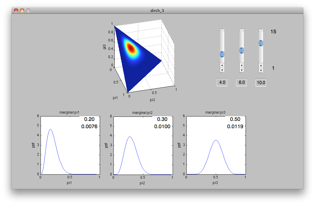
In order to help the graduate students visualize the Dirichlet Process, I made a widget in Matlab that plots the joint PDF of a third order Dirichlet Process. The density is colormapped onto a three dimensional representation of the sample space, which for this case is the plane x+y+z=1, confined to the first quadrant.

A third order Dirichlet Process deals with a random process that has three discrete outcomes, but the probabilities for those outcomes are unknown. The Dirichlet Process quantifies the possible spread of probabilities for the outcomes. Note that each of the three unknown probabilities x, y, and z have to be between 0 and 1, and that x + y + z = 1 (because the sum of probabilities in a sample space always equals one).

You can download the widget (including another version for the 2nd order Dirichlet Process) by clicking here. From within Matlab, just run "dirch_3" or "dirch_2". The smaller plots at the bottom show the marginal densities for the individual variables.

These demos show 2nd and 3rd order processes only because we can physically render them on a computer. Of course mathematics allows us to expand the Dirichlet Process up to n dimensions using all the same concepts and intuition that apply to the 2nd and 3rd order cases, even though creating visualizations of them is impossible.

Neat Coding Trick # 3

Here's the final useful coding trick I learned last week. While Matlab is unparalleled for rapid prototyping, there are any number of reasons why you might want to deploy your code in another language such as C/C++. For example, you might be targeting an embedded device that requires C/C++. Or you might just want to port and compile certain functions you've written in Maltab. This would be the case if you've written a function that is slow to execute in Matlab but that will run very quickly once compiled. Just about anything that is loop-intensive will fall into this category.

For a while now I've known about "mex" functions. Mex functions are C/C++ routines which you compile at the Matlab command line; mex functions must include a special function called mexFunction which specifies how data is passed back and forth between Matlab and the C routine. Once the code is compiled, you call the function from Matlab just as if it were a Matlab function and hopefully you realize huge savings in execution time. This technique works pretty well but the downsides are (a) You have to write the code yourself from scratch and (b) you have to write the mexFunction interface which is tricky at best.

Happily, I discovered "emlc"which generates C code from Matlab code. Here's how it works.

1. Write a function in Matlab
2. Use emlc to convert that code to C from the command line.

Wasn't that easy? There are a few important options that are worth being aware of. Suppose your function is "myFunc.m". You could go to the command line and type:

• emlc -T MEX myFunc

In this case,  your myFunc.m would be converted into myFunc.mexmaci64 (or some other extension depending on your operating system). Your code is automatically ported over and compiled. So you can do all your prototyping in Matlab and then use this simple command to get a high speed executable.

If you are targeting an embedded system and you just need the raw C code, you can instead try using:

• emlc -T RTW

There are a host of options; I recommend reading the emlc documentation to be aware of all the options.

Here are a couple of useful tricks I've learned by trial and error. Most importantly, whereas Matlab will dynamically allocate memory for you on the fly, C/C++ is not set up to do the same and must be explicitly instructed on how to handle memory. For example, suppose you've written a function that takes as input an array "y" which will have two elements in it. Whereas Matlab will give you the benefit of the doubt that "y" will in fact have two elements at run time, C will not. To avoid a compile-time error, you must include the following statement just after your Matlab function heading:

• assert(all(size(y)==[2,1]));

This command tells the compiler to throw a run-time error if the "y" input to the function is not exactly of dimensions two rows and one column.

Along the same lines, you must also pre-allocate all output variables. If your output variable is "dy" and you expect it to have two elements, you can't just say:

• dy(1) =  ... ;
• dy(2) =  ... ;

Instead, you have to say:

• dy = zeros(2,1); % preallocate
• dy(1) =  ... ;
• dy(2) =  ... ;

I also learned that its not good enough to preallocate with an indefinite number. For example, this will cause a compile-time error:

• function dy = myFunc(y,tmax)
• int nPts = tmax/0.001;
• dy = zeros(nPts,1);

The problem is that the compiler has no idea how many points nPts will be. The workaround is to preallocate up to some maximum worst-case array length and then to truncate it as necessary:

• function dy = myFunc(y,tmax)
• int nPts = tmax/0.001;
• int ptsMax = 1e6;
• dy = zeros(ptsMax,1);
• dy(1) = ... ;
• dy(2) = ... ;
• dy = dy(1:nPts);

Finally, you need to include the following comment next to your function heading: %#eml. This facilitates the creation of the compilation report:

• function dy = myFunc(y,tmax) %#eml

Just for kicks, I coded up a single-cell Hodgkin-Huxley simulation using Forward Euler. The point was to create something slow and lumbering so that I could really see the speed difference. You can download the mFile by clicking here.

I used the following command at the Matlab prompt:

• clear; tic; [v,t] = hodgkin_huxley(10,1,100); toc; plot(t,v);

Over five trials, the average elapsed time is 62ms.

Then I converted the m file to a mex file using the steps outlined above and reran it using exactly the same command line command:

• emlc -T MEX hodgkin_huxley
• clear; tic; [v,t] = hodgkin_huxley(10,1,100); toc; plot(t,v);

Now the average elapsed time is 14ms. Thats an execution-time reduction of over 75%, and all it cost me was typing in a single line a the command prompt.

Neat Coding Trick # 2

My Day of Coding last Friday turned up a really useful trick for passing data between Matlab and C/C++ during execution. Suppose you have some C++ code and lots of data, and you want to visualize or otherwise examine your data during runtime either to debug your code or just to make sure that things are happening the way you think they are. Matlab has provided tools to allow you to do just that: pass data from C/C++, during runtime, to Matlab. There, the data can be visualized or otherwise manipulated, and even sent back to C++. Not too bad.

The basic steps are:

• include engine.h - this is an include file that automatically installs with Matlab
• define an "engine" pointer, which opens up a portal between C++ and Matlab
• define Matlab-friendly data elements (mxArrays) for porting your data to Matlab
• stuff data into the Matlab-friendly data elements
• instruct C++ to send the Matlab-friendly data elements to Matlab
• instruct C++ what commands to execute on the data

There are of course more sophisticated options; see Matlab online documentation for more details.

I've put together a brief video outlining the technique. The code shown in the video can be downloaded from here: http://www.box.net/shared/xmazi14uv2