Dirichlet Process Clustering

We've been looking at Dirichlet Process Clustering recently as a great data-driven approach for learning patterns in data. This discussion is about as lucid of a discussion on the topic as I've seen.

(Note, following this link might require that you become a registered user at quora.com - which is an awesome site that you should follow anyways...)

Popular Mechanics!!!

My recently graduated PhD student Alessandro Napoli got himself a nice interview in Popular Mechanics magazine. Check it out!

Pendulum Waves

I did this just for fun. Not a great use of my time but I learned a few neat tricks in the process. I wrote a Matlab simulation of a pendulum art project I saw online.

The original video I based my simulation on is here:

Not that you care, but the Matlab code can be downloaded by clicking here.

Numerical Simulation

The other day I came across a neat problem that I'd used to teach the basics of numerical simulation to some undergraduates a few summers ago. I thought I'd re-post it here. The goal is to solve for the solution to the following third order differential equation:'

• y''' + 5y'' + 8y' + 4y = 1

Use a timestep of dt = 200us and run the simulation for t = 10 seconds. The initial conditions are:

• y(0) = 5
• y'(0) = 1
• y''(0) = 0

This problem is fun because you can solve for a closed form solution and then compare that hand-solved answer to the simulated version. The simulated solution can be run using Matlab, C, or a combination. The combination solution is neat because it uses Matlab to create the data and plot the solution, but uses C-code (compiled in Matlab as a mex-function) as the super-fast solution engine. Mex-Functions are a bit tricky to learn but can often lead to valuable speed-ups in simulations.

The solution to the third order differential equation can be solved by hand. You should get the following function:

The plot for this function is shown below along with the iterated solution that I generated using C++:

Simulated Solutions

Here I present three numerical (i.e. simulated) solutions to the third order differential equation. All three yield the same simulated plot (see blue curve above).

Matlab-Only Solution

clear; 

clf;

dt = 200e-6;

tMax = 10;

nSamples = tMax/dt;

y = zeros(nSamples,1);

a = 1;

b = 0;

y(1) = 5;

for i=2:nSamples

    dy = a;

    da = b;

    db = -8*a - 5*b - 4*y(i-1) + 1;

    y(i) = y(i-1) + dy*dt;

    a    = a      + da*dt;

    b    = b      + db*dt;

end

t = (1:length(y))*dt;   

plot(t,y);

Using the tic/toc commands in Matlab, I determined that the Matlab-only solution took an average of 12ms, including the time to create the plot.

C++ Only Solution

The C++ Only solution is fast, but we need a way to pass the data back to Matlab in order to plot it. In this solution, C++ writes the data to a binary file. Then a separate Matlab script reads the data from the file and plots it.

#include <iostream>
#include <cmath>
#include <fstream>
using namespace std;
int main()
{
double dt = 200e-6;
        double tmax = 10;
double pi = 4 * atan(1);
int    nSamples = floor(tmax/dt);
double da,db,dy;
double a=1;
double b=0;
double y[nSamples];
int i;
ofstream out("data2.bin",ios::out|ios::binary);
y[0] = 5;
for(i=1;i<nSamples;i++){
dy = a;
da = b;
db = -8*a - 5*b - 4*y[i-1] + 1;
y[i] = y[i-1] + dy*dt;
a    = a      + da*dt;
b    = b      + db*dt;
}
out.write((char *)&dt , sizeof(double));
out.write((char *)y  ,nSamples*sizeof(double));
out.close();
return 0;
}

This is the Matlab plot code:

clear;clf
fid = fopen('data2.bin','rb');
dt  = fread(fid,1,'double');y   = fread(fid,'double');
fclose(fid);
t = (0:length(y)-1)*dt;
plot(t,y);xlabel('time (s)');title('Solution to 3rd Order Diff-Eq');

C++ / Matlab / Mex Solution

While the previous solution works, it requires that we switch back and forth between the Matlab and C++ environments, which is inherently inefficient; it also requires that we generate a large data file for the purpose of shuttling the data back and forth. A better solution is to create a mex-file. A mex file is a C/C++ file that is compiled directly within Matlab. The compiled executable can be called directly from Matlab; data parameters can be passed back and forth from Matlab to the executable without the intermediate step of dumping it in a file. This solution requires that we only work with one programming environment: Matlab. The coding is a bit more complicated, but the solution is ultimately more elegant. The complexity of the coding is primarily due to the way Matlab passes data to C/C++. The Matlab data comes in structures, with pointers everywhere; learning to maneuver in this manner takes some getting used to. There are good references for this process here and here.

#include <mex.h>
#include <string.h>
#include <math.h>
// This is the subroutine that actually performs the simulation
void runSim(double **py, double **pt, double dt, double tMax, int *nSamples){
    double pi = 4 * atan(1);
    double da, db, dy;
    double a=1;
    double b=0;
    int i;
    double tTemp = dt;
    double *y, *t;
   
    *nSamples = floor(tMax/dt);
    *py = new double[*nSamples];
    y = *py;
   
    *pt = new double[*nSamples];
    t = *pt;
   
    y[0] = 5;
    t[0] = dt;
    for(i=1;i<*nSamples;i++){
        dy = a;
        da = b;
        db = -8*a - 5*b - 4* y[i-1] + 1;
       
        y[i] = y[i-1] + dy*dt;
        a    = a      + da*dt;
        b    = b      + db*dt;
       
        t[i] = t[i-1] + dt;
    }
}
// ****************************************************
// ******************** START HERE ********************
// ****************************************************
// Mex routines must always start with "mexFunction"
// Here, the input data is imported from Matlab. Then the actual function
// executed (in this case "runSim"), and finally the output data is
// exported back to Matlab
void mexFunction(int nlhs, mxArray *plhs[], int nrhs, const mxArray *prhs[]) {
    // Step 1: Import input variables from Matlab
    double dt   = *(double *)mxGetData(prhs[0]);
    double tMax = *(double *)mxGetData(prhs[1]);
    // Step 2: Declare variables
    int nSamples;
    double *y,*t;
   
    // Step 3: Run the simulation
    runSim(&y, &t, dt, tMax, &nSamples);
   
    // Step 4: Export the results back to Matlab
    double *output;
    if (nlhs>=1){
        plhs[0] = mxCreateDoubleMatrix(nSamples, 1, mxREAL);
        output = mxGetPr(plhs[0]);
        memcpy(output, y, nSamples*sizeof(double));
    }
    if (nlhs>=2){
        plhs[1] = mxCreateDoubleMatrix(nSamples, 1, mxREAL);
        output = mxGetPr(plhs[1]);
        memcpy(output, t, nSamples*sizeof(double));
    }
   
    // Step 5: Housekeeping
    delete [] y;
    delete [] t;
} 

Once the C/C++ code has been written and compiled, the function is called from Matlab in the same way that any other function would be. In this case, the C file was called "diff_eq3.cpp", so therefore the compiled executable is called using "diff_eq3". This simulation took an average of 2ms, including plotting time. That is 6x faster than the Matlab-only solution!

clear; clf;
dt = 200e-6;
tmax = 10;
[y,t] = diff_eq3(dt,tmax);
plot(t,y); 

Convolution

It seems that no matter how long I teach signal processing, I always learn something new. Last week I thought of an interesting experiment regarding convolution and I was pretty surprised by the results. Consider a first order low pass filter with system response H(s) = wc / (s+wc) [where wc is the cutoff frequency in rads/sec]. The impulse response of this system is h(t) = wc*exp(-wc * t), and the corresponding differential equation is y' + wc*y = wc*x.

Suppose we are interested in using a computer to determine the system output y(t) in response to an input x(t). I reasoned that there are two ways of solving this problem. The first is to apply convolution: x(t) [conv] h(t). The second is to use numerical approximation such as Forward Euler to solve the differential equation. In this case, FE could be used to arrive at y[i] = y[i-1](1-wc*dt) + x[i-1](wc*dt), where "dt" is the timestep.

My big "aha" was the realization that there are two competing methods for numerically solving y(t), and in theory they should both give the same answer. However it seems reasonable that one method should be more "efficient" than the other in that it would work better with a larger value of dt (generally speaking you want to use the largest dt you can get away with to reduce your simulation time).

So I decided to test the two methods against each other. My results for simulating a first order step response are shown here:

I've used a pretty large dt in order to accentuate weaknesses of the two approaches. The input step x(t) is in blue and the true (expected) step response y(t) is in black. The green signal shows the answer as computed via convolution whereas the red signal is the answer as computed using Forward Euler. In this case, you can easily see that that Forward Euler/differential equation approach is much more accurate than the convolution method. Of course, if you make dt get smaller and smaller, eventually, both the green and red signals converge onto the true "black" signal.

So then I decided to repeat this experiment with a second order low underdamped low pass filter. Amazingly, the results were reversed!

In this case, the convolution method was much more accurate at low dts than the Forward Euler method. What's going on here? My suspicion is that it has to do with the complexity of the impulse response, which in this case is rather oscillatory, especially as compared to the first order case. My feeling is that the convolution method is better suited for capturing all those oscillations than the Forward Euler method, which is using an estimate of the derivative to capture those oscillations - I think that estimate becomes less accurate for large dt faster than the corresponding calculation of h(t) used in the convolution.

So I thought all this was really interesting! Based on my observations, I hypothesize that (a) for an overdamped 2nd order system, the Euler method would be more accurate than convolution, and (b) for anything higher than a 2nd order system, the convolution method would be more accurate. I've run out of time to test either of these but let me know if you'd like to give it a try. I'd be happy to post your solutions!

Dirichlet Distribution

I'm taking part in a journal club on data modeling comprised of faculty and graduate students. We have started with the paper, "Modeling individual differences using Dirichlet Processes" by Navarro et al. Part of the paper reading process is to delve into the mathematical background that underpins the authors' research, which is how we wound up having a lively discussion on what the Dirichlet Process is and why its important.

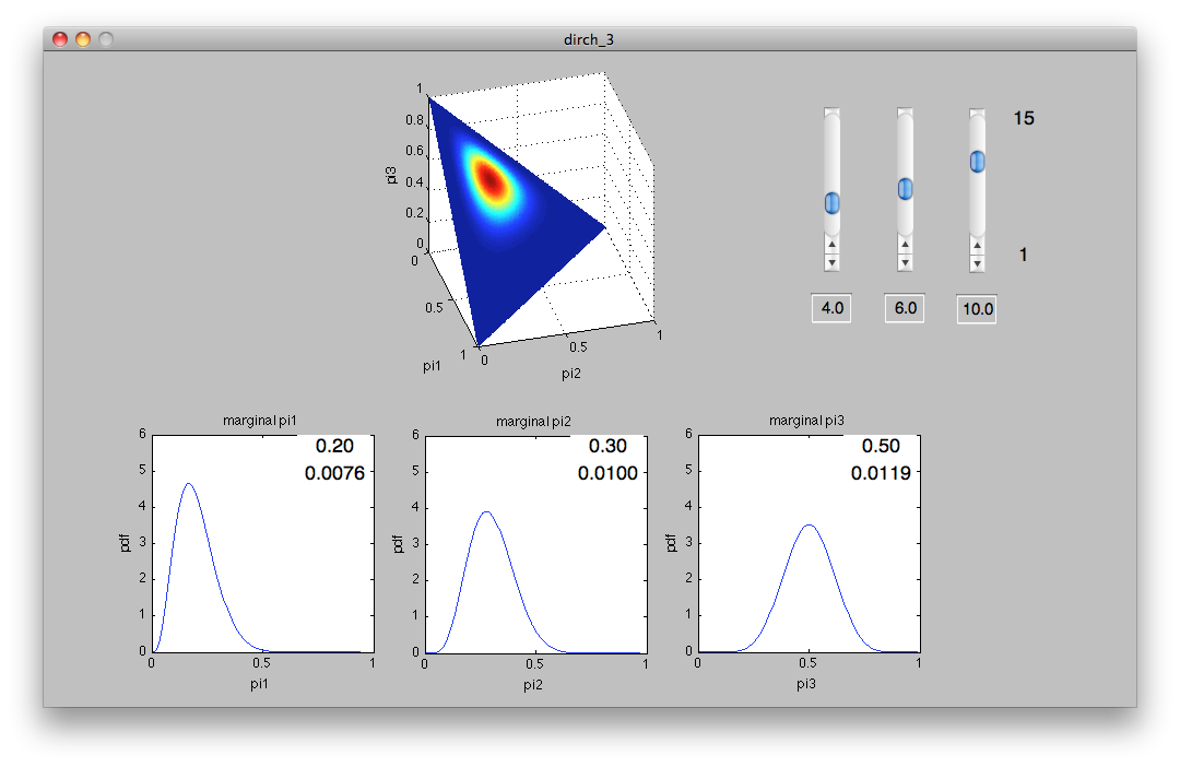
In order to help the graduate students visualize the Dirichlet Process, I made a widget in Matlab that plots the joint PDF of a third order Dirichlet Process. The density is colormapped onto a three dimensional representation of the sample space, which for this case is the plane x+y+z=1, confined to the first quadrant.

A third order Dirichlet Process deals with a random process that has three discrete outcomes, but the probabilities for those outcomes are unknown. The Dirichlet Process quantifies the possible spread of probabilities for the outcomes. Note that each of the three unknown probabilities x, y, and z have to be between 0 and 1, and that x + y + z = 1 (because the sum of probabilities in a sample space always equals one).

You can download the widget (including another version for the 2nd order Dirichlet Process) by clicking here. From within Matlab, just run "dirch_3" or "dirch_2". The smaller plots at the bottom show the marginal densities for the individual variables.

These demos show 2nd and 3rd order processes only because we can physically render them on a computer. Of course mathematics allows us to expand the Dirichlet Process up to n dimensions using all the same concepts and intuition that apply to the 2nd and 3rd order cases, even though creating visualizations of them is impossible.

Neat Coding Trick # 1

Last Friday, I learned three neat coding tricks which I'm going to try to share here. The first one involves inherited classes in C++ and the use of virtual functions to create run-time decisions about which versions of a function to run. This is a very powerful trick because it simplifies function calls and data handling in situations where you have a number of related classes.

I've put together a little demonstration here to illustrate how useful this technique is:

---

#include<iostream> 
using namespace std;

class base {
protected:
 int x;
public:
 void setX(int val){x = val;};
 int getX(){return x;};
 virtual void incrX() = 0;
};

class derived1 : public base {
public:
 void incrX(){x+=1;};
};

class derived2 : public base {
public:
 void incrX(){x+=2;};
};

int main(){

 base *myVars[2];

 myVars[0] = new derived1;
 myVars[1] = new derived2;

 myVars[0]->setX(0);
 myVars[1]->setX(0);

 myVars[0]->incrX();
 myVars[1]->incrX();

 cout << myVars[0]->getX() << endl;
 cout << myVars[1]->getX() << endl;

 delete myVars[0];
 delete myVars[1];

 return 0;
}

---

We can think of this code as implementing two versions of a common class. The "common" portions of the class are in the base class. The base stipulates a private variable named x, as well as functions for setting and retrieving x. The base also stipulates an undefined virtual function named incrX. The way I've coded, this, any derived class that inherits base must define its own implementation of incrX. In the "derived1" class, incrX increments the value of "x" by 1, whereas in "derived2", incrX increments the value of x by 2.

In the main function, I create an array of pointers of type *base. I can then create new instances of the derived class and have those pointers stored in the array of type *base. This is a pretty amazing trick. Because derived1 and derived2 both inherit base, I am allowed to define a pointer of type *base and point it to either of the derived classes.

The second remarkable part of this code is that when I run the myVars[0]->incrX() command, the code is clever enough to realize that myVars[0] actually points to an object of class "derived1"; it then runs the appropriate version of incrX.

This trick is very handy because it is going to allow us to solve a few nasty problems in our neuron simulator. We have models for about five basic neuron types. In many ways, those neuron types are similar: all must keep track of who their pre-synaptic neurons are and all must have a function for numerically updating the state variables. However in other ways, those neurons are quite different: the differential equations and state variables are all different from neuron to neuron.

The elegant solution to this model is to create a "base" neuron which contains all the elements that are common to all neurons. The base neuron will also stipulate a virtual "update" function which will need to be redefined by each specific neuron type. Then we can create five "derived" classes which inherit the base and add the individual update functions and state variables. The great part is that in the "main" function, I only have to maintain a single array of neurons. I do this by creating an array of pointers of type *base. Then I can populate that array with any combination of the five neurons. When I tell a neuron to "update", the program makes sure that the update function appropriate to the specific neuron is called.

Another neat upshot of this technique is that the base neuron class can contain a vector of pointers to base which can be populated with pointers to presynaptic neurons, regardless of their specific type.

Thanks to Chris for figuring most of this out!

C++ Performance Benchmarking

We are in the process of developing computational models of neural structures with the eventual goal of studying the effects of deep brain stimulation on dystonia. We are starting by reproducing the results of one of the best-recognized models of neural tissue in the deep-brain, published in 2004 by Rubin and Terman. That paper draws heavily from an earlier 2002 paper which describes some of the basic neural cell models. I have an exceptionally capable student who has been working with these models for a while now and has successfully re-created each of the individual cell types; we are now working on linking those cells together synaptically and optimizing the simulation process.

The neural models used by Rubin and Terman are Hodgkin-Huxley-type which means that each of the voltage-gated membrane proteins is modelled by one or more differential equations. For example, in the case of the Subthalamic Neuron cells, there are seven first-order differential equations that must be solved in parallel.

Numerically, there are any number of methods for solving these differential equations. The most simple are Forward Euler and Runge-Kutta, each of which use a mathematical approximation of the derivative to iteratively determine the next value of the solution, given the current value of the solution. More advanced methods such as Runge-Kutta-Fehlberg and Runge-Kutta Prince-Dormand use adaptive time-stepping, which means they exploit the fact that you can solve the differential equation less often when the signal isn't changing so much in time. Of course, there is a computational overhead involved with calculating what the optimal time-step is, which  might temper some of the advantage of adaptive-timestepping.

I decided to run a sample simulation on a few different computers to determine how fast the simulations are running. I ran an array of 100 subthalamic neurons (each with seven differential equations) for 2500ms under a variety of conditions. Not that it matters, but the neurons were independent; there was no interneuron connectivity for this test. All code was written in C++ using the GSL library for solving the differential equations.

I ran two tests: (1) which simulation method is better, and (2) how fast are the various computers we are using.

Test 1
Using our fastest computer (a dedicated processing-only workstation; see below for more details) I simulated the 100-neuron model using three different differential equation solvers.

Method	Timestep Type	Execution Time	Points Generated
Runge-Kutta 4	Fixed	147.7s	250,000
Ruge-Kutta-Fehlberg	Adaptive	4.86s	10,237
Runge-Kutta Prince-Dormand	Adaptive	5.7s	4,558

The RKPD method produces by far the fewest number of data points, but takes about 17% longer to execute that the fastest method, RKF.

Test 2
The simulation was repeated of five different computers; the RKF simulation was used in every case.

Computer	Specs	Execution Time
Dedicated Linux Workstation	3.2GHz Quad Core i7, 6GB RAM	4.86s
iMac (2009)	3.06GHz Core 2 Duo, 4GB RAM	5.40s
Mac Mini (2011)	2.4GHz Core 2 Duo, 2GB RAM	6.88s
Macbook Pro (2007)	2.4GHz Core 2 Duo, 4GB RAM	7.21s
Old Laptop*	2.2GHz Core 2 Duo, 4GB RAM	17.45s

*The "old laptop" simulation was actually run on virtual Ubunutu box running on the old laptop under Windows...

The first test is interesting because it emphasizes the tradeoff between fewer number of points versus longer simulation time. The second test demonstrates that our new dedicated Linux machine is actually quite fast, even when compared with other reasonably fast machines.

Its important to work through some of these issues while the simulations are still relatively small; understanding the tradeoffs now will be very helpful when the simulations get up to thousands or even tens of thousands of neurons.

GNU Science Library

In our quest to get better and running simulations of networks of neurons, we've been trying to replicate a number of papers covering a variety of techniques. For example, we looked at the integrate-and-fire model of Hansel 1998 and the modified Hodgkin & Huxley approach of Rubin and Terman 2004.

Part of the problem in running these simulations is developing and properly understanding the numerical methodology responsible for cranking through the differential equations. There are a number of available techniques, and up until now we'd been basically hand coding them (we're developing our simulations in GNU C/C++ since we want these sims to run quickly over tens of thousands of neurons, which basically rules out Matlab). Forward Euler is pretty easy to code but is numerically very limited and requires small step sizes (meaning large numbers of calculations). More advanced methods such as Runge-Kutta and the adaptive step-size method of Runge-Kutta-Fehlberg can get away with far fewer calculations but require more coding and are therefore more prone to coding mistakes. All that extra code has to be tested and validated, a time consuming process.

We were pleased then to discover that the GNU Science Library (or GSL for short) has built in support for Ordinary Differential Equations. Although I'd used GSL before because of its matrix library (which its cumbersome to use - I now prefer to use openCV's matrix library instead), I hadn't been aware of its ODE capabilities. The solver supports a range of algorithms including the embedded Runge-Kutta Prince-Dormand method and the august Bulirsch-Stoer method that actually required a Jacobian in addition to the actual differential equations themselves.

If I have some time later this week I'll post some benchmarks to give an idea on the savings of computation time.